Implement style transfer with VGG19

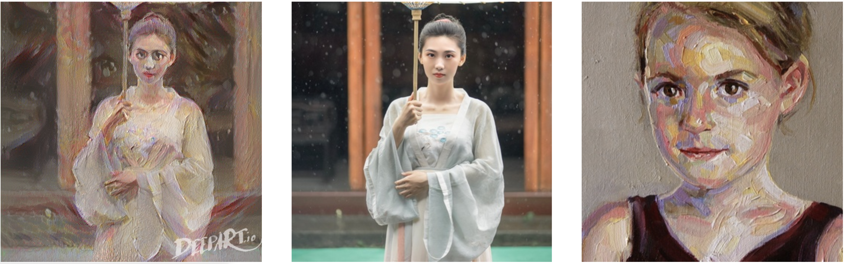
An example of style transfer is shown in the header image. This was made by a web app. It looks like this is a bit overtrained. You can try it out with your own image! If it does not look good, you might want to fine tune the parameters a bit.

In order to understand different structures stored in feature maps, I’ll implement a style transfer manually, using method that is outlined in the paper Image Style Transfer Using Convolutional Neural Networks written by Gatys.

In this paper, style transfer uses the features found in the 19-layer VGG Network, which is comprised of a series of convolutional and pooling layers, and a few fully-connected layers. In the image below, the convolutional layers are named by stack and their order in the stack. Conv_1_1 is the first convolutional layer that an image is passed through, in the first stack. Conv_2_1 is the first convolutional layer in the second stack. The deepest convolutional layer in the network is conv_5_4.

Separating Style and Content

Style transfer relies on separating the content and style of an image. Given one content image and one style image, we aim to create a new, target image which should contain our desired content and style components:

• objects and their arrangement are similar to that of the content image
• style, colors, and textures are similar to that of the style image

I’ll use a pre-trained VGG19 to extract content or style features from a passed-in image. I’ll then quantify content and style losses and use those to iteratively update the target image. The following walkthrough code was copied from Udacity deep learning repo.

---

Load in VGG19

VGG19 is split into two portions:

• vgg19.features, which are all the convolutional and pooling layers
• vgg19.classifier, which are the three linear, classifier layers at the end

We only need the features portion, which we’re going to load in and “freeze” the weights of, below.

from PIL import Image
import matplotlib.pyplot as plt
import numpy as np
import torch.optim as optim
from torchvision import transforms, models

vgg = models.vgg19(pretrained=True).features

for param in vgg.parameters():
    param.requires_grad_(False)

device = torch.device("cuda" if torch.cuda.is_available() else "cpu")

vgg.to(device)

Sequential(
  (0): Conv2d(3, 64, kernel_size=(3, 3), stride=(1, 1), padding=(1, 1))
  (1): ReLU(inplace)
  (2): Conv2d(64, 64, kernel_size=(3, 3), stride=(1, 1), padding=(1, 1))
  (3): ReLU(inplace)
  (4): MaxPool2d(kernel_size=2, stride=2, padding=0, dilation=1, ceil_mode=False)
  (5): Conv2d(64, 128, kernel_size=(3, 3), stride=(1, 1), padding=(1, 1))
  (6): ReLU(inplace)
  (7): Conv2d(128, 128, kernel_size=(3, 3), stride=(1, 1), padding=(1, 1))
  (8): ReLU(inplace)
  (9): MaxPool2d(kernel_size=2, stride=2, padding=0, dilation=1, ceil_mode=False)
  (10): Conv2d(128, 256, kernel_size=(3, 3), stride=(1, 1), padding=(1, 1))
  (11): ReLU(inplace)
  (12): Conv2d(256, 256, kernel_size=(3, 3), stride=(1, 1), padding=(1, 1))
  (13): ReLU(inplace)
  (14): Conv2d(256, 256, kernel_size=(3, 3), stride=(1, 1), padding=(1, 1))
  (15): ReLU(inplace)
  (16): Conv2d(256, 256, kernel_size=(3, 3), stride=(1, 1), padding=(1, 1))
  (17): ReLU(inplace)
  (18): MaxPool2d(kernel_size=2, stride=2, padding=0, dilation=1, ceil_mode=False)
  (19): Conv2d(256, 512, kernel_size=(3, 3), stride=(1, 1), padding=(1, 1))
  (20): ReLU(inplace)
  (21): Conv2d(512, 512, kernel_size=(3, 3), stride=(1, 1), padding=(1, 1))
  (22): ReLU(inplace)
  (23): Conv2d(512, 512, kernel_size=(3, 3), stride=(1, 1), padding=(1, 1))
  (24): ReLU(inplace)
  (25): Conv2d(512, 512, kernel_size=(3, 3), stride=(1, 1), padding=(1, 1))
  (26): ReLU(inplace)
  (27): MaxPool2d(kernel_size=2, stride=2, padding=0, dilation=1, ceil_mode=False)
  (28): Conv2d(512, 512, kernel_size=(3, 3), stride=(1, 1), padding=(1, 1))
  (29): ReLU(inplace)
  (30): Conv2d(512, 512, kernel_size=(3, 3), stride=(1, 1), padding=(1, 1))
  (31): ReLU(inplace)
  (32): Conv2d(512, 512, kernel_size=(3, 3), stride=(1, 1), padding=(1, 1))
  (33): ReLU(inplace)
  (34): Conv2d(512, 512, kernel_size=(3, 3), stride=(1, 1), padding=(1, 1))
  (35): ReLU(inplace)
  (36): MaxPool2d(kernel_size=2, stride=2, padding=0, dilation=1, ceil_mode=False)
)

Load in content and style images

Content and Style Features

Map layer names to the names found in the paper for the content representation and the style representation

def get_features(image, model, layers=None):
    """ Run an image forward through a model and get the features for 
        a set of layers. Default layers are for VGGNet matching Gatys et al (2016)
    """
    
    ## Need the layers for the content and style representations of an image
    if layers is None:
        layers = {'0':'conv1_1',
		  '5':'conv2_1',
		  '10':'conv3_1',
		  '19':'conv4_1',
		  '21':'conv4_2',
		  '28':'conv5_1'}

    features = {}
    x = image
    # model._modules is a dictionary holding each module in the model
    for name, layer in model._modules.items():
        x = layer(x)
        if name in layers:
            features[layers[name]] = x
            
    return features

Gram Matrix

The output of every convolutional layer is a tensor with dimensions associated with the batch_size, a depth, d and some height and width (h, w). The Gram matrix of a convolutional layer can be calculated as follows:

• Get the depth, height, and width of a tensor using batch_size, d, h, w = tensor.size()
• Reshape that tensor so that the spatial dimensions are flattened
• Calculate the gram matrix by multiplying the reshaped tensor by it’s transpose

def gram_matrix(tensor):
    """ Calculate the Gram Matrix of a given tensor 
        Gram Matrix: https://en.wikipedia.org/wiki/Gramian_matrix
    """
    
    batch_size, d, h, w = tensor.size()
    ## reshape it, so we're multiplying the features for each channel
    matrix = tensor.view(d, h * w)
    ## calculate the gram matrix
    gram = torch.mm(matrix,matrix.t())
    
    return gram

I’ll extract our features from images and calculate the gram matrices for each layer in our style representation.

# get content and style features only once before forming the target image
content_features = get_features(content, vgg)
style_features = get_features(style, vgg)

# calculate the gram matrices for each layer of our style representation
style_grams = {layer: gram_matrix(style_features[layer]) for layer in style_features}

target = content.clone().requires_grad_(True).to(device)

Loss and Weights

Individual Layer Style Weights

Weight the style representation at each relevant layer. Use a range between 0-1 to weight these layers. By weighting earlier layers (conv1_1 and conv2_1) more, you can expect to get larger style artifacts in your resulting, target image. Should you choose to weight later layers, you’ll get more emphasis on smaller features. This is because each layer is a different size and together they create a multi-scale style representation!

Content and Style Weight

Just like in the paper, I define an alpha (content_weight) and a beta (style_weight). This ratio will affect how stylized your final image is. It’s recommended that to leave the content_weight = 1 and set the style_weight to achieve the ratio.

style_weights = {'conv1_1': 1.,
                 'conv2_1': 0.8,
                 'conv3_1': 0.5,
                 'conv4_1': 0.3,
                 'conv5_1': 0.1}

content_weight = 1  # alpha
style_weight = 1e6  # beta

Updating the Target & Calculating Losses

Inside the iteration loop, calculate the content and style losses and update target image accordingly.

The content loss will be the mean squared difference between the target and content features at layer conv4_2. The style loss is calculated in a similar way, only you have to iterate through a number of layers, specified by name in the dictionary style_weights. Finally, create the total loss by adding up the style and content losses and weighting them with your specified alpha and beta.

# for displaying the target image, intermittently
show_every = 400

optimizer = optim.Adam([target], lr=0.003)
steps = 2000  # decide how many iterations to update 

for ii in range(1, steps+1):
    
    ## get the features from your target image    
    ## Then calculate the content loss
    target_features = get_features(target, vgg)
    content_loss = torch.mean((target_features['conv4_2'] - content_features['conv4_2'])**2)
    
    # the style loss
    # initialize the style loss to 0
    style_loss = 0
    # iterate through each style layer and add to the style loss
    for layer in style_weights:
        # get the "target" style representation for the layer
        target_feature = target_features[layer]
        _, d, h, w = target_feature.shape
        
        ## Calculate the target gram matrix
        matrix = target_feature.view(d, h * w)
        target_gram = torch.mm(matrix,matrix.t())
        
        ## get the "style" style representation
        style_gram = style_grams[layer]
        ## Calculate the style loss for one layer, weighted appropriately
        layer_style_loss = style_weights[layer] * torch.mean((target_gram - style_gram)**2)
        
        # add to the style loss
        style_loss += layer_style_loss / (d * h * w)
        
        
    ## calculate the *total* loss
    total_loss = style_weight * style_loss + content_weight * content_loss
    
    # update your target image
    optimizer.zero_grad()
    total_loss.backward()
    optimizer.step()
    
    # display intermediate images and print the loss
    if  ii % show_every == 0:
        print('Total loss: ', total_loss.item())
        plt.imshow(im_convert(target))
        plt.show()

For every 400 steps, you can see that total loss decrease by some amount. You can decide how many steps to take.

Finally, display the result

fig, (ax1, ax2) = plt.subplots(1, 2, figsize=(20, 10))
ax1.imshow(im_convert(content))
ax2.imshow(im_convert(target))

Does this look better? For the whole “training process”, check out my repo.

Reference: Udacity deep learning repo